

Big O notation questions are very popular interview questions for companies who are looking to find talented and promising candidates. Graduates can very easily miss out on an amazing career opportunity if they are not well revised with the topic. While there are plenty of cheat sheets out there to help jog your memory, this post is intended as a guide to help introduce or revise the basics of Big O.
Understanding Big O notation is a good first step towards designing good functions, alogirthms and complex systems. It is a relative mathematical representation to describe the complexity a given algorithm’s upper bound. In simple terms an algorithm will take no more than ‘this’ many steps to complete and allows us to compare it one to another algorithm. What we measure using Big O is not fixed, we can apply Big O notation to describe any independent criteria such as Memory usage, CPU usage and can also show the trade off of these criteria. For the purposes of this post I will express these criteria as “operations” or “operational cost”.
Big O can be a good tool to compare scalability (growth) of a algorithm, function or system. Big O is used to find the upper bound of an algorithm, we can combine it with Big Omega (lower bound) to give us Big Theta (tight bound) which would give us a combination of both upper and lower bounds. Below is a quick breakdown of what bounds mean.
Big O – An algorithm will take no more than ‘this’ many steps to complete.
Big Omega – An algorithm will take at least ‘this’ many steps to complete.
Big Theta – An algorithm will take exactly ‘this’ many steps to complete.
Please note this is not a system to compare the best case average case and worst case scenarios each one of the Big X’s can express its own best, worst and average case. We’re going to be sticking to Big-O for this post as upper bounds is a good place to start.
Big O
Before jumping into code and testing, I’d like to make a list of classes of functions that are commonly encountered. The most scalable are listed first and the worst are at the bottom. I have omitted a few from the list but have included them near the bottom of this post.
Notation Name
O(1) Constant
O(log n) Logarithmic
O(N) Linear
O(N2) Quadratic
O(2N) Exponential
To better illustrate the differences a graph is a good graphical representation of the notations above. click here if the image below is not clear or cannot be viewed.
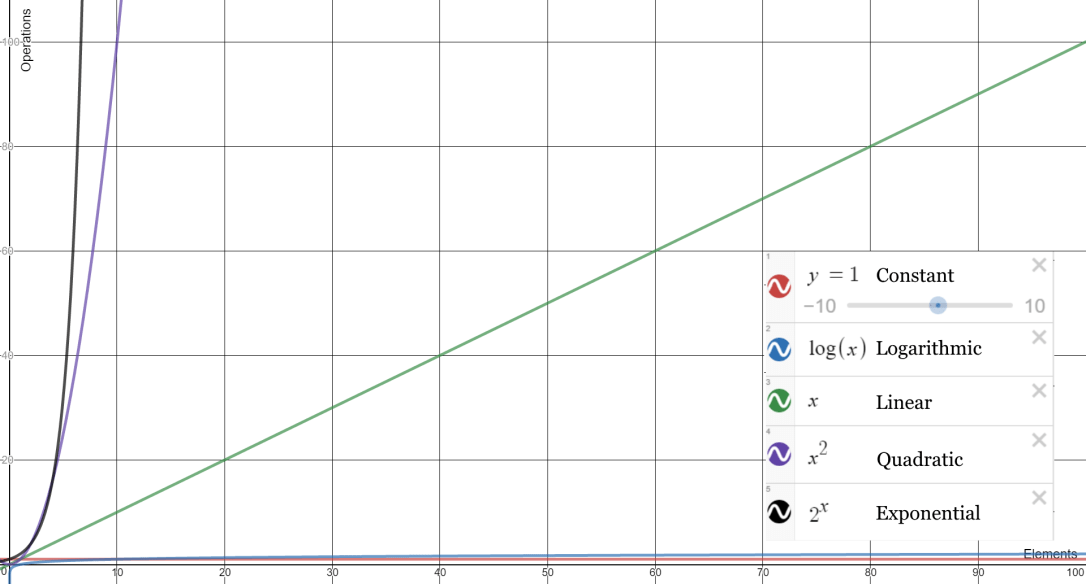
Constant
Constant will always have the operation remain at a constant regardless of how many elements you have. For example given a dataset of 1 it will take 1 operation. if we increase the items to 10, 100 or 1000 the operational cost will always be 1. It behaves the same no matter what.
Logarithmic
In logarithmic complexity the operational cost does increase with the size of the data set. However the relationship between elements and operations are not proportional. This makes logarithmic algorithms very scalable. It may not be clear in the graph above, but logarithmic scaling means that a data set of 10 may have an operational cost of 1. 100 takes two seconds. 1000 takes 3 seconds and so on.
Linear
This one is the easiest to remember. The growth in data is directly proportional to the growth in operation expense. If the data set grows by a given factor the operation time will also increase by the same factor. A data set of 10 would take 10 operations, 20 would take 20 operations. 30 would make 30 and so on.
Quadratic
Having an algorithm that completes at this this point and beyond are very bad at scaling. A data set of 1 would have a cost of 1, 10 would cost 100, 100 would cost 10000. Its clear here that the rate in which the operational cost grows is very quick to the number of elements.
Exponential
For each new element you add here the operational cost will increase by a factor of 2. This means 1 item will take 1 second. 2 would be 2. 3 would be 9. 4 is 16. by the time we get to 10 the operational cost has grown to 1024, by 100 the cost would be 1,267,650,600,228,229,401,496,703,205,376. An example I like to give to exponential growth is folding a piece of paper in half again and again. The world record at the time of writing this is 13 and thats using industrial toilet paper taped together at 1.2km long. This means that the end product has 8192 layers. Looking back at our previous example, 10 folds would have produced 1024, by increasing our elements by two we will have increased the cost by a factor of 8.
More examples
To reduce cluttering the graph I limited the number of examples given, below are some more classes of functions.
Log Linear – O(n log n)
Log linear would sit between Linear and Quadratic, this can be expressed with O(n log n). This is slower then Linear alone as the operational cost would increase at proportional plus a logarithmic rate. A data set of 1 would take 2 operations, 10 items takes 12 and 100 would be 103.
Cubic – O(N^3)
Cubic would sit between Quadratic and Exponential. It increases operational cost at a rate of the number of elements cubed. 13 is 1. 103 would be 1000 and 100 would be 1,000,000. notice how cubic is very similar to quadratic.
Factorial – O(N!)
Factorial would sit at the very end of the list after Exponential. It grows faster than exponential.
